Algorithmic Musical Genre Classification

(A detailed write-up of this project can be found here, and the code is publicly available on GitHub.)

Summary

In this project, I construct a data pipeline which intakes raw .wav files, and then uses machine learning to predict the genre of the track. We first do a frequency-space transformation (similar to the Fourier transform), and then do randomized dimension reduction on the resulting array. Finally, we put the dimension-reduced signal through a naive Bayes classifier, which we train on about 500 sample tracks.

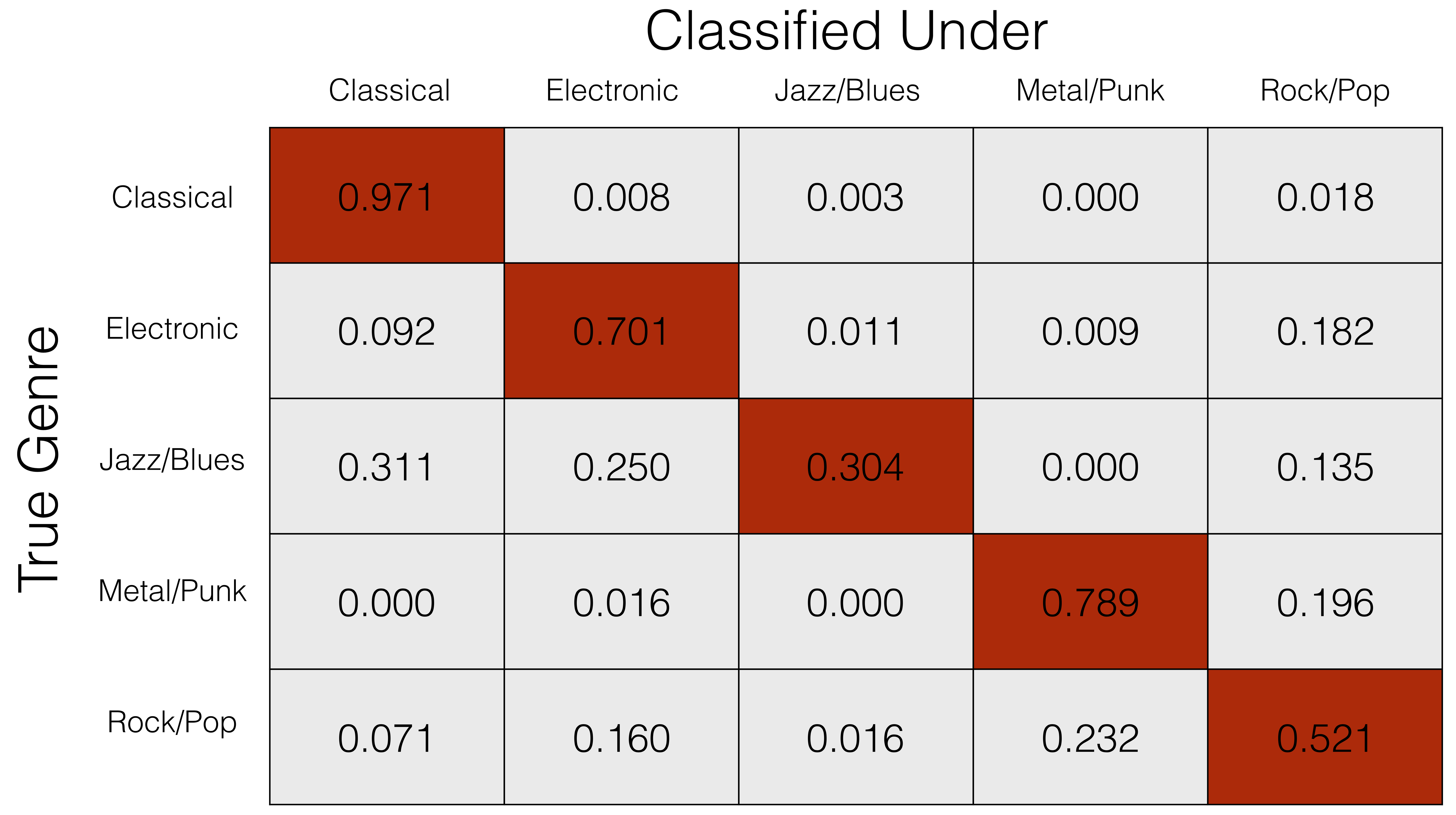
Below is the confusion matrix for the resulting classifier. As one might expect, classical is pretty easy; jazz is hard. A more thorough discussion of the algorithm and results, including additional (less successful) approaches, can be found below.

Introduction

A few years ago I designed a machine learning algorithm which performs automatic genre classification of musical signals. The basic idea is that if the genre of a piece of music has certain acoustic signatures, then a computer should be able to pick up on those. However, teasing out those signatures requires some signal processing know-how, along with some knowledge of data preprocessing and classification methodologies from the machine learning domain.

We consider five genres: classical, jazz/blues, electronic, metal/punk, and rock/pop. This taxonomy is far from exhaustive, but is a good starting point, with genres that are for the most part quite acoustically distinct. Our most efficient model classifies with 80% accuracy. Those interested can read the full write-up of the project; here I’ll go through the big ideas and leave out the details.

Preprocessing

We begin with a raw .wav file, which is an uncompressed format for storing audio signals.¹ We then remove the beginning and end of the track, as songs often start and end with indiosyncratic structures that are not indicative of the genre.

Next, we perform a spectral decomposition. This means we decompose the signal into its frequency components. When you look at the display on an equalizer and see the signal bars at different frequencies, you are looking at a spectral decomposition.

The most common spectral decomposition in mathematics and physics is the Fourier Transform. However, the Fourier Transform does not efficiently represent how the human ear hears sound; we hear frequencies on a logarithmic scale, meaning that if notes are one octave apart, then the frequency of the second is twice the frequency of the first.² To mitigate this issue, we use the mel-frequency cepstrum, which is naturally logarithmically scaled. We now have a frequency decomposition, which we expect to be useful in analyzing sound; for example, we expect classical music to have lower signal at the bass frequencies compared to electronic music.

After obtaining the time-varying mel-frequency cepstrum components (MFCCs), we have a time series of about 1000 points, with each point having 30 coefficients. Said another way, our musical track now lives in a 30,000 dimensional space. We are thus up against the ubiquitous problem of machine learning, the curse of dimensionality.

Dimensionality Reduction

The mathematics surrounding the analysis of high-dimensional data is rich and fascinating. One remarkable result is that you can perform entirely random (!) projections, reducing the dimensionality by orders of magnitude, and still retain most of the information present in the data. This result is known to mathematicians as the Johnson-Lindenstrauss Lemma.

The beauty of this result is twofold. The geometry and analysis behind it are surprising, yet intuitive once grasped; also, it immediately provides us with a dimensionality-reduction algorithm which is computationally efficient and trivial to implement.³

There are, of course, other more sophisticated approaches to the problem of dimensionality reduction. The ubiquitous principal component analysis (PCA) is a projection method, but it selects the projections based on their explanatory power. The Johnson Lindenstrauss lemma is telling us, essentially, that when our data is high dimensional we don’t need to worry about which direction we choose; all directions, with high probability, will contain most of the signal present in the data.⁴

Graph Representations

As a more high-falutin alternative to random projections, we explore dimensionality methods based on graph embeddings. A graph (also called a network) is a collection of objects and their connections. The details of this approach become quite technical, so this presentation will be qualitative rather than quantitative.

Recall that, for each track, we now have a time series of points in 30-dimensional space, or equivalent 30 time series in one dimensional space). Each dimension represents a frequency band. We build a graph by considering interactions between these bands;⁵ does the intensity of the low frequencies tend to move with the intensity of high frequencies? Or, are their intensity profiles independent?

So, for each possible pair of our 30 frequency bands (435 possible pairs in total), we have a pairwise term indicating the interaction strength. We then perform a final embedding which reduces our graph into a vector in 30 dimensions. This embedding is based on the eigenvalues of the matrix represntation of the graph, and a description of it is beyond the scope of this article; suffice to say, it is the same technique that lies at the heart of Google’s PageRank algorithm, and is a well-tested method for graph embedding.

Classification

We now have two competing models, both of which result in data of a reasonable dimension (30 dimensions vs 30,000). But we still face the task of classifying these data points into groups. In our case, since we will train our model on labelled training data, we are looking at a supervised learning scenario.

We compare the efficacy of two approaches: a naive Bayes classifier, and a support-vector classifier. The first is a linear model, so it does not consider pairwise interation terms between data features (i.e. the dimensions of our data points). This simplicity makes the model computationally efficient and highly interpretable, but for some data the interaction terms are very important, and a model such as naive Bayes will not have optimal performance.

The support-vector machine approach is more computationally intensive than that of naive Bayes. However, it is able to model arbitrary interactions between data features, depending on the kernel chosen. We use a radial basis function (RBF) kernel, which models nonlinear interactions in a localised way, and is known to be effective in a variety of settings.⁶

Results

Below are accuracy plots and confusion matrices for both the random projection and graph embedding techniques.

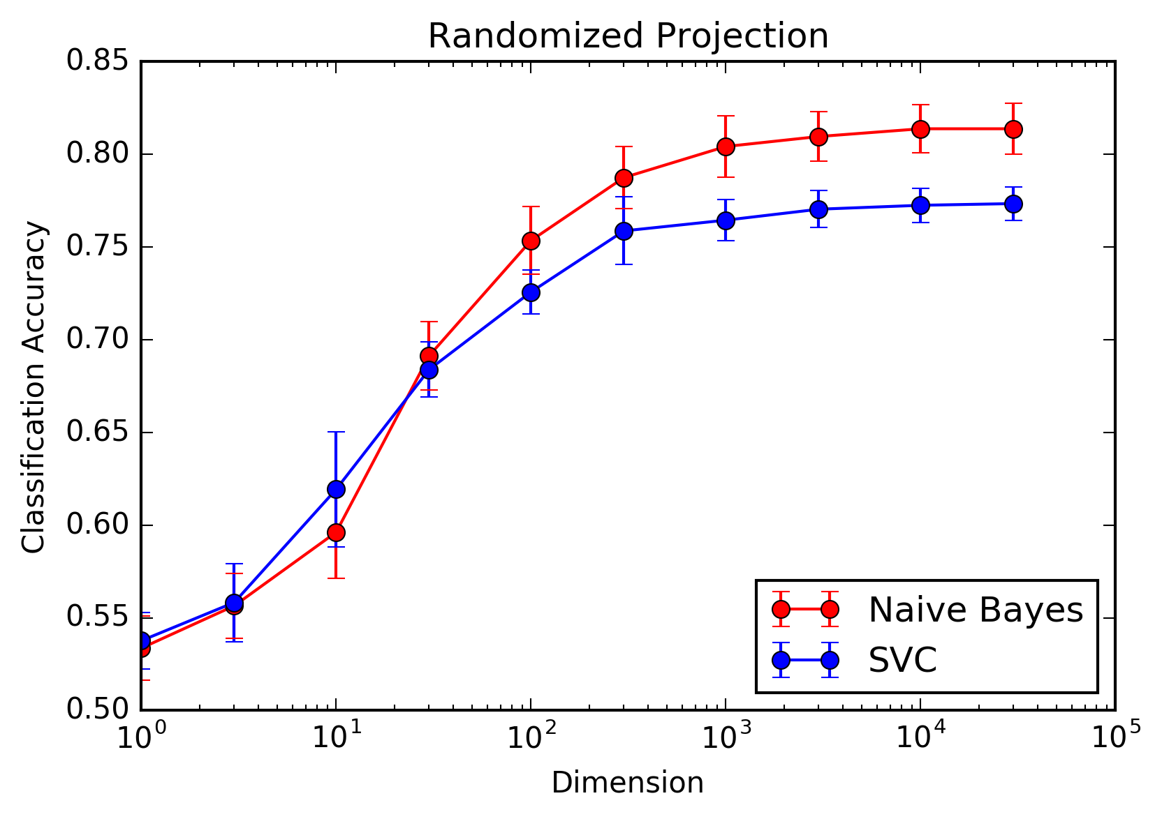
The first pair of charts are for the randomized projection model. Based on what we see, we recommend using a Naive Bayes classifier with \(\approx 10^3\) dimensions. This is the optimal balance of performance and computational efficiency, obtaining 98% performance relative to the problem without any dimensionality reduction. Interestingly, the support vector classifier underperforms Naive Bayes, indicating that the interaction terms between features contain more noise than signal.

Things are quite different when we use graph embedding as our dimensionality reduction method. In this case, there is in fact an optimal number of dimensions, and increasing beyond this optimal dimensionality has a significant detrimental effect on performance. This is to be expected, as our spectral embedding method naturally chooses the more informative dimensions first, and later features have a lower signal to noise ratio.

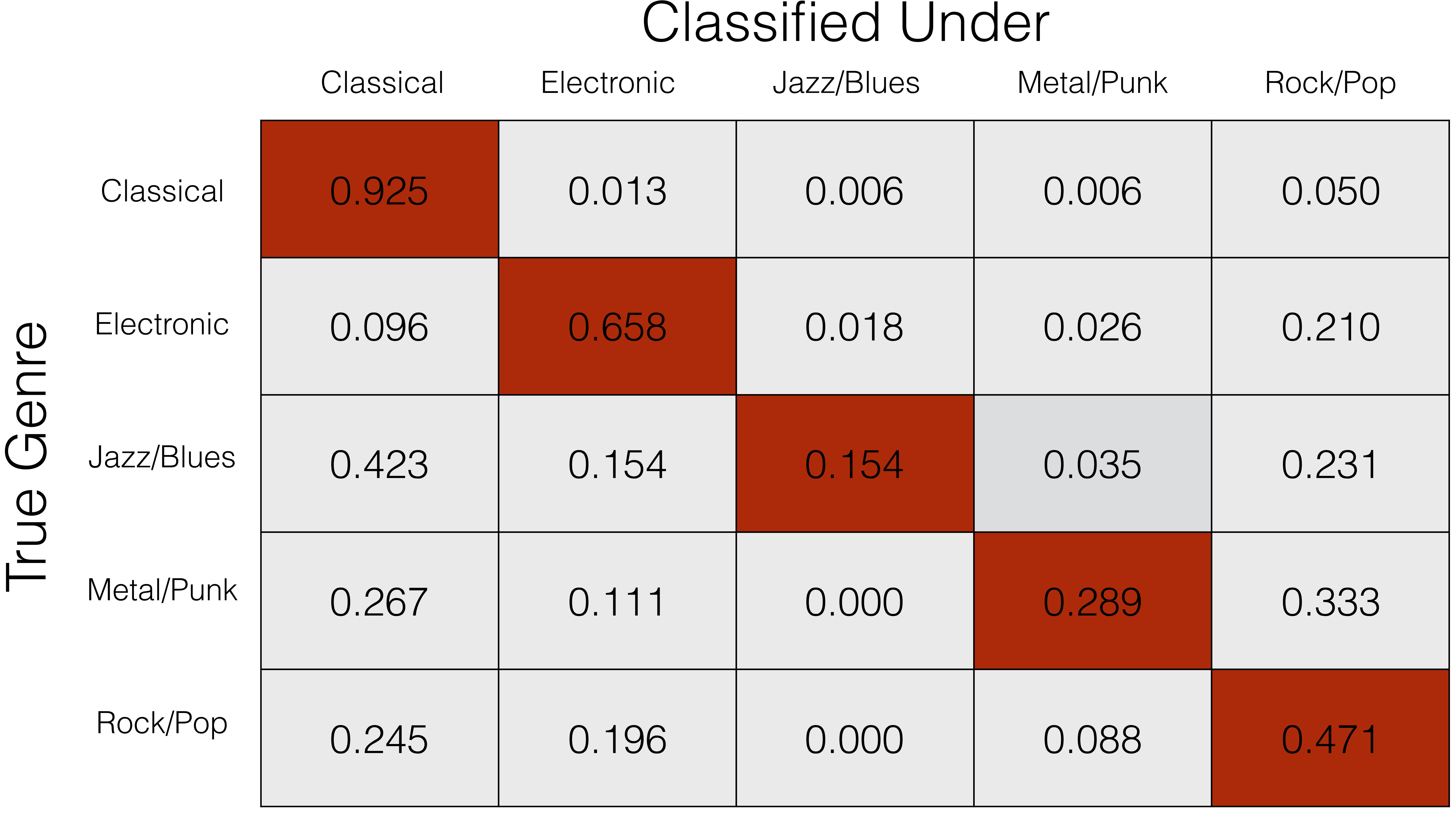
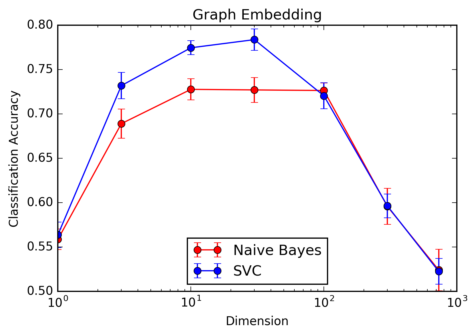
When using graph embedding, the support vector classifier outperforms the naive Bayes classifier, indicating that interaction terms in our spectral embedding are much more informative than they are in our random projection. Again, this implies that the structural information in the spectral embedding is both front-loaded and has complicated interdependence structure, whereas the random projection method generates mostly independent features which are, on average, of equal importance.

In both scenarios, we see that the easiest genre to classify is classical, and the hardest is jazz/blues. This is what we would expect, since classical has a distinct acoustic signature (i.e. instrumentation), while jazz/blues is highly variable, and such a wide variety of training data will not produce an accurate classifier.

Conclusion

The key takeaway from this project is that simple methods often work very well. The optimal approach relied on the simpler dimensionality reduction technique (random projections) and the simpler classifier (naive Bayes). This simplicity gives the added benefit of computational efficiency and model interpretability.

1. Most common compression methods, such as .mp3 and .aac, rely on decomposing the signal into its frequency components, and removing the high frequency components, which are primarily noise and/or inaudible to the human ear. We’ll end up doing a frequency decomposition of our own later on, as described below. ↩

2. In contrast, if we heard sound on a linear scale, then the frequency of the second note would be some fixed amount above the first. ↩

3. We simple generate a large, orthogonal matrix \(\mathbf{Q}\) which, when multiplied by our data matrix, projects the data points into a lower-dimensional space. Thus, the cost of the projection is the cost of generating this matrix (random number draws) and the cost of a matrix-matrix multiply (which can be performed efficiently when the involved matrices are sparse). ↩

4. The seemingly paradoxical nature of this statement is apparent; how can any direction contain most of the information? The geometry of high dimensions is very strange, and not something human minds are well-designed to consider intuitively. For the curious, a good place to begin puzzling is the phenomenon of concentration of measure, which says that most of the material in a ball gets closer to the edge of the ball as the dimension that the ball lives in gets higher. ↩

5. We use Perason correlation to measure the interaction between the time series, but this is far from the only choice. ↩

6. See the Wikipedia entry for the RBF kernel for more information. ↩