Anomaly Detection in Dynamic Networks
(This section is an overview of material available as a preprint on the arXiv.)
Introduction to Network Data
“Data analysis” is a hugely popular thing these days, for obvious reasons. When most people think of “data,” they think of a table where the columns are variables and the rows are observations:
| Name | Age | Height | Weight |
|---|---|---|---|
| Fred | 28 | 6’0” | 190 |
| Sally | 24 | 5’8” | 145 |
| Jimmy | 52 | 5’6” | 160 |
| Nicole | 61 | 5”11” | 155 |
We might call this “tabular data.” We are interested in an alternate form of data called “networked data,” which stores connections between entries (people, computers, etc.). The canonical example of network data is a social network. If arranged in a table, we would see both rows and columns labelled with names, and entries are marked if the two names are linked in a given social network (e.g. are “friends” on Facebook).
| User | Fred | Sally | Jimmy | Nicole |
|---|---|---|---|---|
| Fred | X | X | ||
| Sally | X | X | ||
| Jimmy | X | X | X | |
| Nicole | X |
Such data is often visualized with each user as a dot (called a vertex) and each connection as a line (called an edge). The resulting object is called a network.1 The table above corresponds to the network seen below:
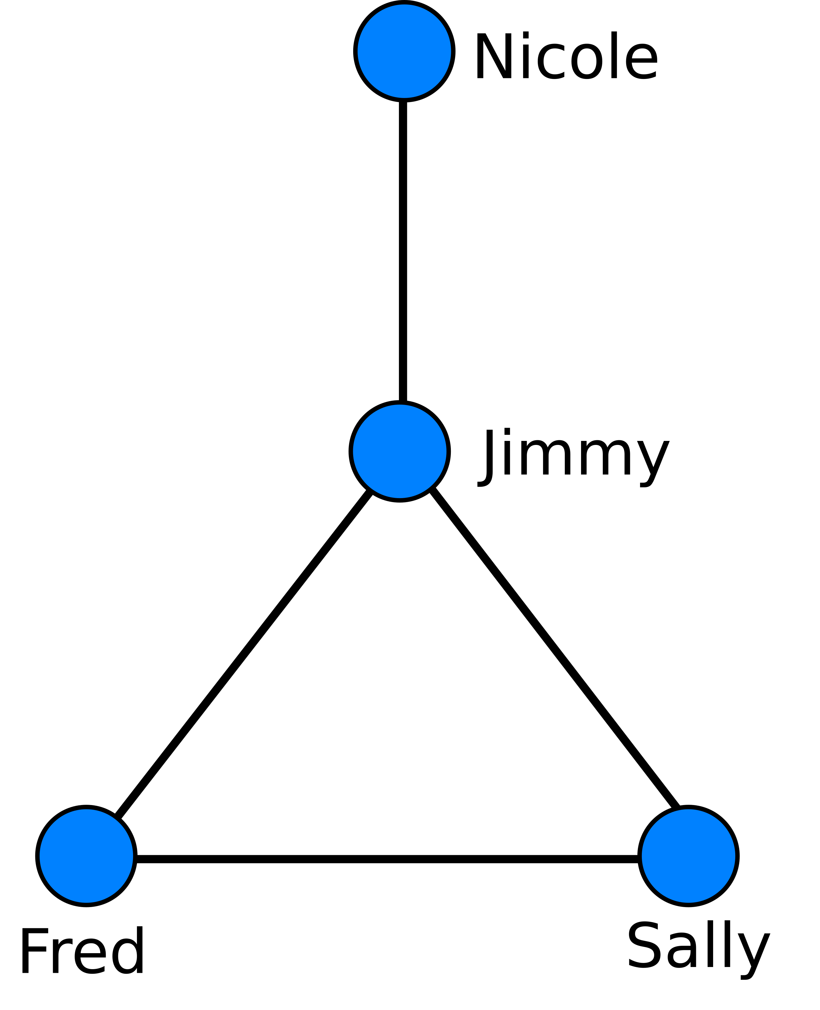
Looking at this network, we see that the different people have different “roles,” so to speak. Jimmy is central, acting as a hub; he is friends with all other members of the network. Nicole is an outlier, so that information moving around the network might take longer to reach her than other members. Fred, Sally, and Jimmy form a clique, or tightly knit group in which everyone is connected to everyone else.
This sort of analysis is fundamental to the kind of insights that people want to get out of network data. Are their communities? How many? Significant hubs? Are certain groups outliers, or are most of the groups reasonably well connected? Answering these questions is simple for graphs small enough to draw as we have above; they are quite challenging for graphs with millions of nodes.
The Resistance Metric
My first focus in graph analysis was the “graph resistance,”1 one of many ways to quantify the “distance” between two vertices on a graph. Probably the most obvious way to measure distance between two vertices is to calculate the length (number of edges) of the shortest path between them. Foe example, in the image above, the shortest path between Nicole and Sally goes through Jimmy, and has length 2.
This approach is appealing in its simplicity, but has its drawbacks. In the road network of New York City, for example, the shortest path between Brooklyn and Manhattan is the same as the shortest path between Brooklyn and Queens. But as anyone who’s been to New York knows, if you’re in a car during rush hour, you’d much rather be driving on the latter route. This is because there are very few ways to get from Brooklyn to Manhattan; you must cross one of a small number of bridges. The shortest path distance fails to take these multiple routes into account.
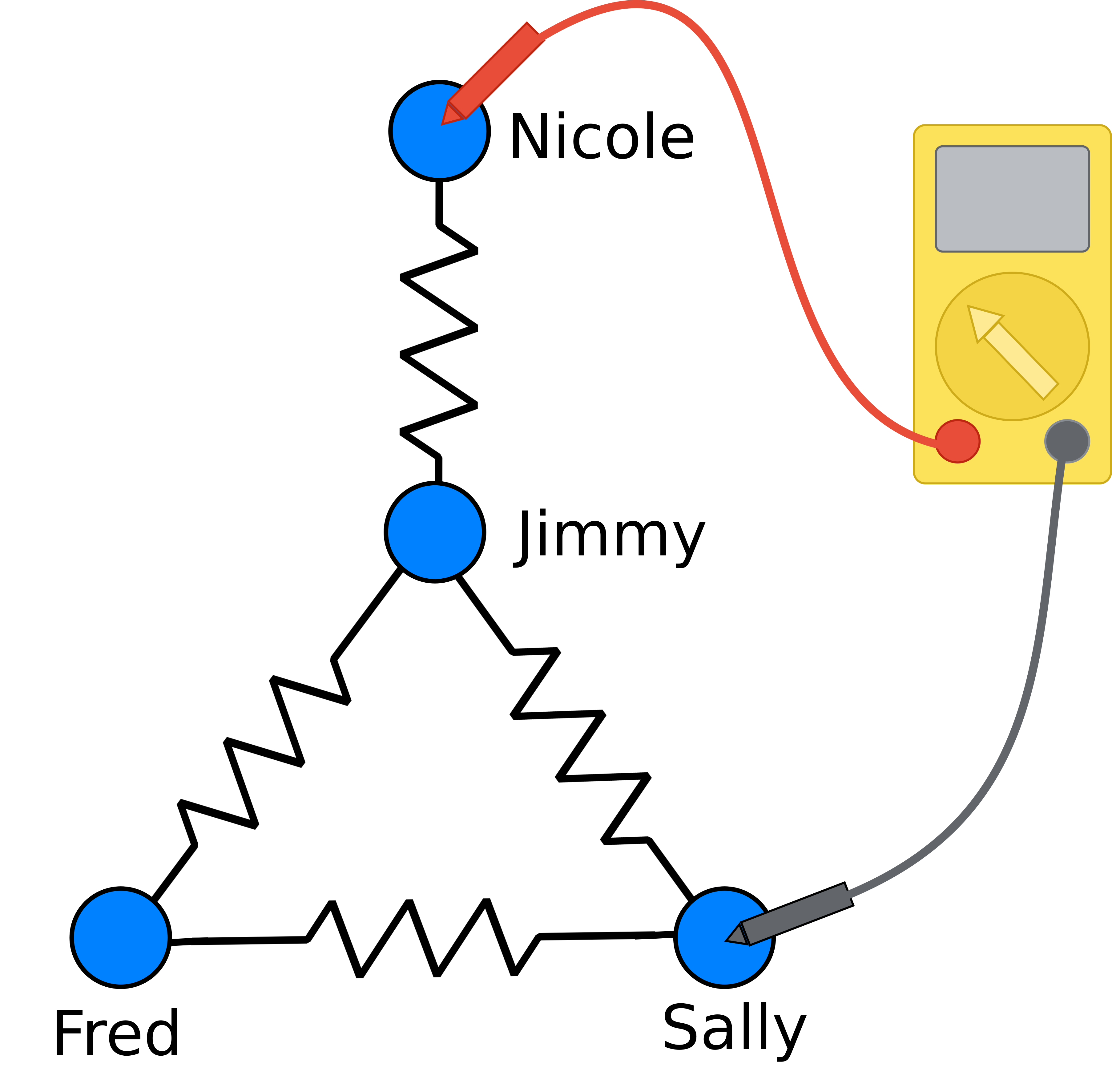
The graph resistance treats the network like a set of resistors, and measures the “distance” between two vertices by measuring the appropriate resistance.2 Resistance is determined by all possible paths that electricity can flow through a network; in this way the graph resistance takes into account all possible paths between the two vertices. In our previous example, Brooklyn and Manhattan would have a much higher resistance than Brooklyn and Queens, because there are very few paths between them.
In our paper, we extend this idea into a method of comparing two graphs by looking at their resistance structure, and prove some results about the ability of the graph resistance to detect changes in communities. In particular, we focus on using the tool for anomaly detection in networks that change over time (see the next section for more details), and explore the limiting cases of sparse network structure where this tool starts to break down. In particular, we find theoretical limits in which the resistance can detect changes in the community structure of a graph.
Dynamic Anomaly Detection
Using the graph resistance isn’t the only method for comparing graphs. After our last work I was very interested to compare the various method, to see how our theoretical analysis of the resistance translates into the real world and compares to other metrics. Since network data is very often big data, we focus on fast distances, where the time taken scales linearly with the size of the network.3
I’ll focus here on the particular case of anomaly detection in dynamic networks, which are networks that change in time.4 Think of a social network changing in time; we might want to know when this social network undergoes “important” change. An example of an important change would be if two friend groups merged into a single indistinguishable group. In contrast, and unimportant change would be if a few friendships were added or removed between people already members of the same friend group.
One of the experiments we’ve performed involves analysis of a social network of primary school students in France, recorded in 2009. The students wear RFID tags that record if they are in close contact, and then we can build a network where the vertices are students, and the edges indicate contact between two students.
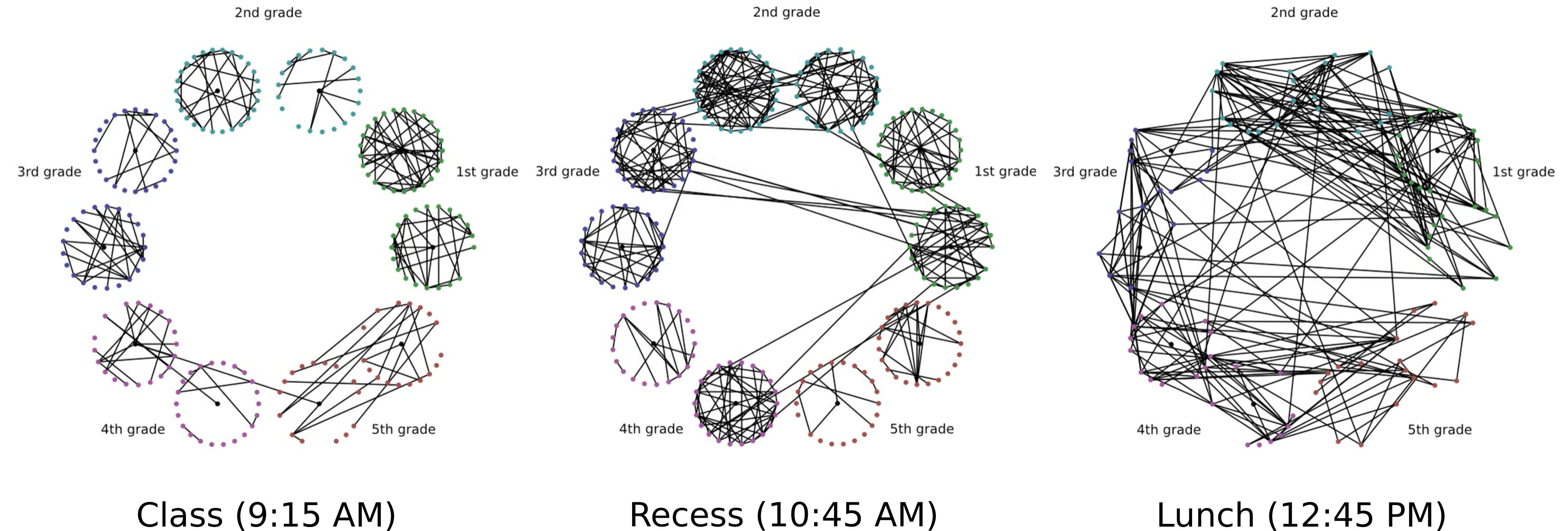
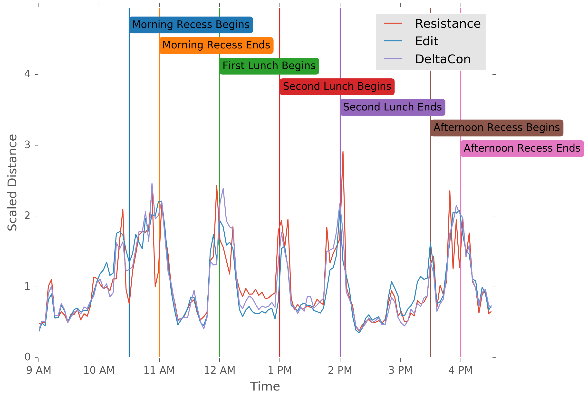
This graph changes over time, undergoing important structural changes during recess and lunch. The students form exclusive groups during class time, as they are restricted to their classrooms. During recess, they mainly play with classmates, but a significant amount of cross-class contact also occurs. In lunch, the class-group becomes almost entirely insignificant. But which distances will most effectively pick up on this difference?
Our comparison shows that the resistance distance is comparable in performance to both the industry-standard edit distance and the cutting-edge DeltaCon distance in identifying these anomalous times, and frequently outperforma, albeit at the cost of increased variability. We also examine spectral methods,5 but we find that their performance is so noisy that they do not effectively identify the anomalous times in the graph.
A realistic anomaly detection scheme would employ an ensemble of models, and compare and constrast the information from each. Although I’ve only shown one of our many experiments here, the work taken in its entirety gives a thorough understanding of the strengths and weaknesses of a wide variety of fast distance techniques, and guides the user in applying them to real-world data problems.
-
Mathematicians refer to networks as graphs, while the term network is more common with computer scientists. I find the latter to be more descriptive, so I’ll stick to using it. ↩ ↩2
-
For a more technical introduction, and an excellent overview of basic properties, see the paper Effective Graph Resistance. ↩
-
I.e., if the graph is twice as large, it takes twice as long to compute the distance, rather than four or eight times as long. ↩
-
In our upcoming paper, we also look at statistical graph matching, which is comparing a graph to a population and determining the likelihood that this graph is drawn from the population. We do this by examining a number of random graph models, such as preferential attachment, small world, and the stochastic blockmodel. ↩
-
Spectral distances arise from analyzing the matrix representation of a network, and in particular comparing the eigenvalues of these matrices. ↩