Your p-values Are Bogus

People often use a Gaussian to approximate distributions of sample means. This is generally justified by the central limit theorem, which states that the sample mean of an independent and identically distributed sequence of random variables converges to a normal random variable in distribution.¹ In hypothesis testing, we might use this to calculate a \(p\)-value, which then is used to drive decision making.

I’m going to show that calculating \(p\)-values in this way is actually incorrect, and leads to results that get less accurate as you collect more data! This has substantial implications for those who care about the statistical rigor of their A/B tests, which are often based on Gaussian (normal) approximations.

A Simple Example

Let’s take a very simple example. Let’s say that the prevailing wisdom is that no more than 20% of people like rollerskating. You suspect that the number is in fact much larger, and so you decide to run a statistical test. In this test, you model each person as a Bernoulli random variable with parameter \(p\). The null hypothesis \(H_0\) is that \(p\leq 0.2\). You decide to go out and ask 100 people their opinions on rollerskating.²

You begin gathering data. Unbeknownst to you, it is in fact the case that a full 80% of the population enjoys rollerskating. So, as you randomly ask people if they enjoy rollerskating, you end up getting a lot of “yes” responses. Once you’ve gotten 100 responses, you start analyzing the data.

It turns out that you got 74 “yes” responses, and 26 “no” responses. Since you’re a practiced statistician, you know that you can calculate a \(p\)-value by finding the probability that a binomial random variable with parameter \(p_0=0.2\) would generate a value \(k\geq74\) with \(n=100\). This probability is just

\[p_\text{exact} = \text{Prob}(k\geq 74) = \sum_{k=74}^{n}{n \choose k} p_0^{k} (1-p_0)^{(n-k)}.\]

However, you know that you can approximate a binomial distribution with a Gaussian of mean \(\mu=np_0\) and variance \(\sigma^2=np_0(1-p_0)\), so you decide to calculate an approximate \(p\)-value,

\[p_\text{approx} = \frac{1}{\sqrt{2\pi np_0(1-p_0)}}\int_{k=74}^\infty \exp\left(-\frac{(k-np_0)^2}{2np_0(1-p_0)}\right).\]

However, this approximation is actually incorrect, and will give you progressively worse estimates of \(p_\text{exact}\). Let’s observe this in action.

Python Simulation of Data

We simulate data for values \(n=1\) through \(n=1000\), and compute the corresponding exact and approximate \(p\)-value. We plot the log of the \(p\) value, since they get very small very quickly.

from matplotlib import pyplot as plt
import numpy as np
import pandas as pd
from scipy.stats import norm, binom

plt.style.use( ['classic', 'ggplot'])

p_true = 0.8
n = 1000
data = binom.rvs(1, p_true, size=n)
p0 = 0.2
p_vals = pd.DataFrame(
    index=range(1,n), 
    columns=['true p-value', 'normal approx. p-value']
)

for n0 in range(1,n):
    normal_dev = np.sqrt(n0*p0*(1-p0))
    normal_mean = n0*p0
    k = sum(data[:n0])
    # the "survival function" is 1 - cdf, which is the p-value in our case
    normal_logpval = norm.logsf(k, loc=normal_mean, scale=normal_dev)
    true_logpval = binom.logsf(k=k, n=n0, p=p0)
    p_vals.loc[n0, 'true p-value'] = true_logpval
    p_vals.loc[n0, 'normal approx. p-value'] = normal_logpval
    
p_vals.replace([-np.inf, np.inf], np.nan).dropna().plot(figsize = (8,6));
plt.xlabel("Number of Samples")
plt.ylabel("Log-p Value");

We have to drop infs because after about \(n=850\) or so, the \(p\)-value actually gets too small for scipy.stats to calculate; it just returns -np.inf.

The resulting plot tells a shocking tale:

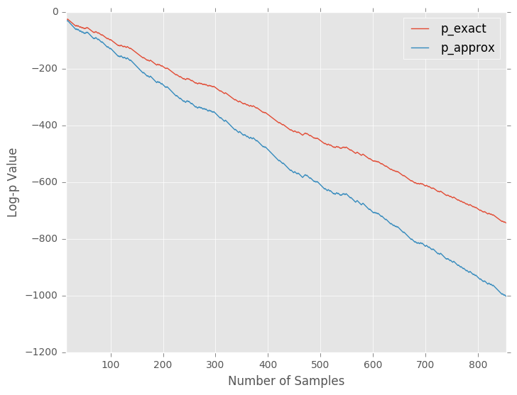
The approximation diverges from the exact value! Seeing this, you begin to weep bitterly. Is the Central Limit Theorem invalid? Has your whole life been a lie? It turns out that the answer to the first is a resounding no, and the second… probably also no. But then what is going on here?

Convergence Is Not Enough

The first thing to note is that, mathematically speaking, the two \(p\)-values \(p_\text{exact}\) and \(p_\text{approx}\) do, in fact, converge. That is to say, as we increase the number of samples, their difference is approaching zero:

\[\left| p_\text{exact} - p_\text{approx}\right| \rightarrow 0\]

What I’m arguing, then, is that convergence is not enough.

If it were, then we could just approximate the true \(p\)-value with 0. That is, we could report a \(p\)-value of \(p_\text{approx} = 0\), and claim that since our approximation is converging to the actual value, it should be taken seriously. Obviously, this should not be taken seriously as an approximation.

Our intuitive sense of “convergence”, the sense that \(p_\text{approx}\) is becoming “a better and better approximation of” \(p_\text{exact}\) as we take more samples, corresponds to the percent error converging to zero:

\[\left| \frac{p_\text{approx} - p_\text{exact}}{p_\text{exact}}\right| \rightarrow 0.\]

In terms of asymptotic decay, this is a stronger claim than convergence. Rather than their difference converging to zero, which means it is \(o(1)\), we demand that their difference converge to zero faster than \(p_\text{exact}\),

\[\left| p_\text{exact} - p_\text{approx}\right| = o\left(p_\text{exact}\right).\]

It would also suffice to have an upper bound on the \(p\)-value; that is, if we could say that \(p_\text{exact} < p_\text{approx}\), so \(p_\text{exact}\) is at worst our approximate value \(p_\text{approx}\), and we knew that this held regardless of sample size, then we could report our approximate result knowing that it was at worst a bit conservative. However, as far as I can see, the central limit theorem and other similar convergence results give us no such guarantee.

Implications

What I’ve shown is that for the simple case above, Gaussian approximation is not a strategy that will get you good estimates of the true \(p\)-value, especially for large amounts of data. You will under-estimate your \(p\)-value, and therefore overestimate the strength of evidence you have against the null hypothesis.

Although A/B testing is a slightly more complex scenario, I suspect that the same problem exists in that realm. A refresher on a typical A/B test scenario: you, as the administrator of the test, care about the difference between two sample means. If they samples are from Bernoulli random variables (a good model of click-through rates), then the true distribution of this difference is the distribution of the difference of (scaled) binomial random variables, which is more difficult to write down and work with. Of course, the Gaussian approximation is simple, since the difference of two Gaussians is again a Gaussian.³

Most statistical tests are approximate in this way. For example, the \(\chi^2\) test for goodness of fit is an approximate test. So what are we to make of the fact that this approximation does not guarantee increasingly valid \(p\)-values? Honestly, I don’t know. I’m sure that others have considered this issue, but I’m not familiar with the thinking of the statistical community on it. (As always, please comment if you know something that would help me understand this better.) All I know is that when doing tests like this in the future, I’ll be much more careful about how I report my results.

Afterword: Technical Details

As I said above, the two \(p\)-values do, in fact, converge. However, there is an interesting mathematical twist in that the convergence is not guaranteed by the central limit theorem. It’s a bit besides the point, and quite technical, but I found it so interesting that I thought I should write it up.

As I said, this section isn’t essential to my central argument about the insufficiency of simple convergence; it’s more of an interesting aside.

Limitations of the Central Limit Theorem

To understand the problem, we have to do a deep dive into the details of the central limit theorem. This will get technical. The TL;DR is that since our \(p\)-values are getting smaller, the CLT doesn’t actually guarantee that they will converge.

Suppose we have a sequence of random variables \(X_1, X_2, X_3, \ldots\). These would be, in the example above, the Bernoulli random variables that represent individual people’s responses to your question about rollerskates. Suppose that these random variables are independent and identically distributed, with mean \(\mu\) and finite variance \(\sigma^2\).⁴

Let \(S_n\) be the sample mean of all the \(X_i\) up through \(n\):

\[S_n = \frac{1}{n} \sum_{i=1}^n X_i.\]

We want to say what distribution the sample mean converges to. First, we know it’ll converge to something close to the mean, so let’s subtract that off so that it converges to something close to zero. So now we’re considering \(S_n - \mu\). But we also know that the standard deviation goes down like \(1/\sqrt{n}\), so to get it to converge to something stable, we have to multiply by \(\sqrt{n}\). So now we’re considering the shifted and scaled sample mean \(\sqrt{n}\left(S_n - \mu\right)\).

The central limit theorem states that this converges in distribution to a normal random variable with distribution \(N(0, \sigma^2)\). Notationally, you might see mathematicians write

\[\sqrt{n}\left(S_n-\mu\right)\ \xrightarrow{D} N(0,\sigma^2).\]

What does it mean that they converge in distribution? It means that, for a fixed area, the areas under the respective curves converge. Note that we have to fix the area to get convergence. Let’s look at some pictures. First, note that we can plot the exact distribution of the variable \(\sqrt{n}(S_n-\mu)\); it’s just a binomial random variable, appropriately shifted and scaled. We’ll plot this alongside the normal approximation \(N(0,\sigma^2)\).

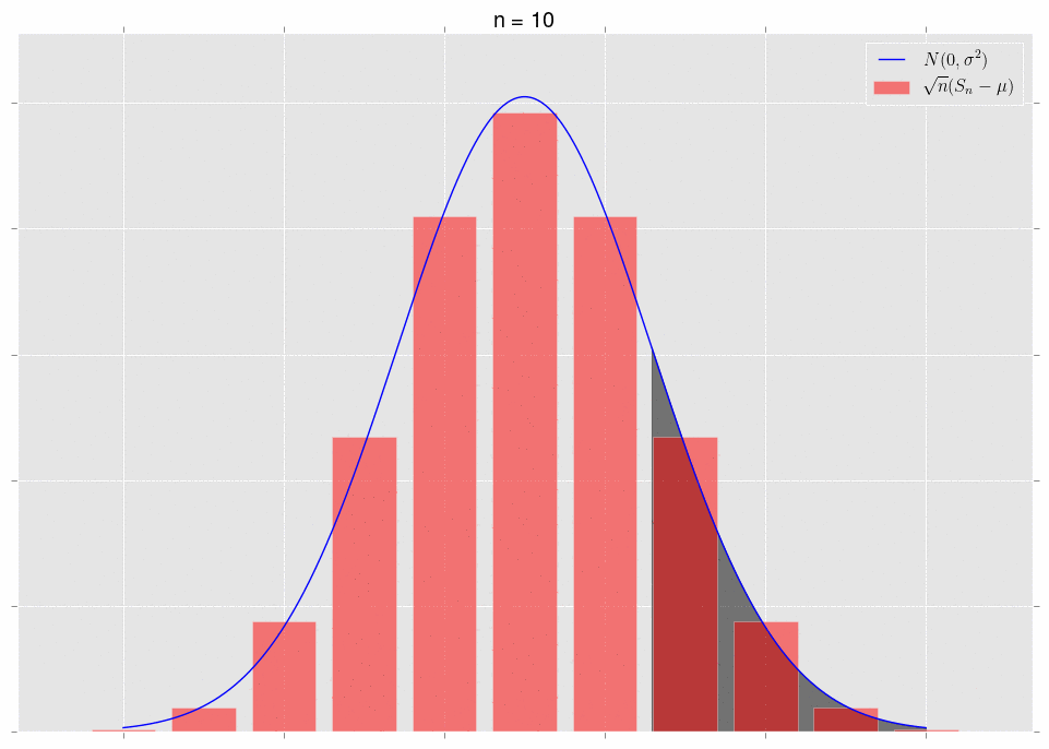
The area under the shaded part of the normal converges to the area of the bars in that same shaded region. This is what convergence in distribution means.

Now for the crux. As we gather data, it becomes more and more obvious that our null hypothesis is incorrect - that is, we move further and further out into the tail of the null hypothesis’ distribution for \(S_n\). This is very intuitive - as we gather more data, we expect our \(p\)-value to go down. The \(p\)-value is a tail integral of the distribution, so we expect to be moving further and further into the tail of the distribution.

Here’s a gif, where the shaded region represents the \(p\)-value that we’re calculating:

As we increase \(n\), the area we’re integrating changes. So we don’t get convergence guarantees from the CLT.

The Berry-Esseen Theorem

It’s worth noting that there is a stronger statement of convergence that applies specifically to the convergence of the binomial distribution to the corresponding Gaussian. It is called the Barry-Esseen Theorem, and it states that the maximum distance between the cumulative probability functions of the binomial and the corresponding Gaussian is \(o(n^{-1/2})\). This claim, which is akin to uniform convergence of functions (compare to the pointwise convergence of the CLT) does, in fact, guarantee that our \(p\)-values will converge.

But, as I’ve said above, this is immaterial, albeit interesting; we know already that the \(p\)-values converge, and we also know that this is not enough for us to be reporting one as an approximation of the other.

1. So long as the variance of the distribution being sampled is finite. ↩

2. You should decide this number based on some alternative hypothesis and a power analysis. Also, you should ensure that you are sampling people evenly - going to a park, for example, might bias your sample towards those that enjoy rollerskating. ↩

3. I haven’t done a numerical test on this scenario because the true distribution (the difference between two scaled binomials) is nontrivial to calcualte, and numerical issues arise as we calculate such small \(p\)-values, which SciPy takes care of for us in the above example. But as I said, I would be unsurprised if our Gaussian-approximated \(p\)-values are increasingly poor approximations of the true \(p\)-value as we gather more samples. ↩

4. In our case, for a single Bernoulli random variable with parameter \(p\), we have \(\mu=p\) and \(\sigma^2=p(1-p)\). ↩